Dispersion relation calculation - field sweeps

This example shows how we can sweep parameters of the dispersion and plot different views on the data. In this example we will use the SingleLayer class based on the Kalinikos-Slavin model [J. Phys. C: Solid State Phys., 19, 7013 (1986)] and plot field dependency of the selected spin wave properties (e.g. mode frequencies and decay lengths) for specified set of k-vectors. The same approach can be used also with other classes available in SpinWaveToolkit.

Let’s start by importing necessary modules and defining material and “experiment” parameters:

#necessary imports
import SpinWaveToolkit as SWT
import numpy as np
import matplotlib.pyplot as plt

# prepare arrays with k-vectors and B-field values of interest
k = np.linspace(0, 10e6, 101) # k-vector values in rad/m,
k[0] = 1e-5 # we use k=1e-5 instead of k=0 to avoid badly conditioned calculations at k=0
B = np.linspace(0, 100e-3, 101) # define values of a field sweep in T
B[0] = 1e-5 # we use B=1e-5 instead of B=0 to avoid badly conditioned calculations at B=0

# Define the experiment geometry
theta = np.pi/2  # (rad) for in-plane magnetization
phi = np.pi/2  # (rad) for Damon-Eshbach geometry

# Define material parameters
# We will use built-in material parameters of NiFe in this example. Built in materials are: (NiFe, YIG, CoFeB, FeNi).
mat = SWT.NiFe
d = 30e-9  # (m) layer thickness
bc = 1 # boundary conditions (1 - totally unpinned, 2 - totally pinned spins)

Calculate dispersions for defined values of external magnetic field

Now we can initiate SWT.SingleLayer and just change the Bext attribute for every field value and store everything in a 2D array.

# Create numpy arrays n0 and decay0 for all fields and k-vectors defined in B and kxi
n0 = [] #initialize list of arrays
decay0 = [] #initialize list of arrays
sl = SWT.SingleLayer(B[0], mat, d, k, theta, phi, boundary_cond=bc)

for index, Bext in enumerate(B):
    sl.Bext = Bext # set external field
    n0.append(sl.GetDispersion(n=0)*1e-9/(2*np.pi)) #Fundamental mode frequency in GHz
    decay0.append(sl.GetDecLen(n=0)*1e6) #Fundamental mode decay length in um
n0 = np.array(n0) # create 2D array from list of arrays
decay0 = np.array(decay0) # create 2D array from list of arrays

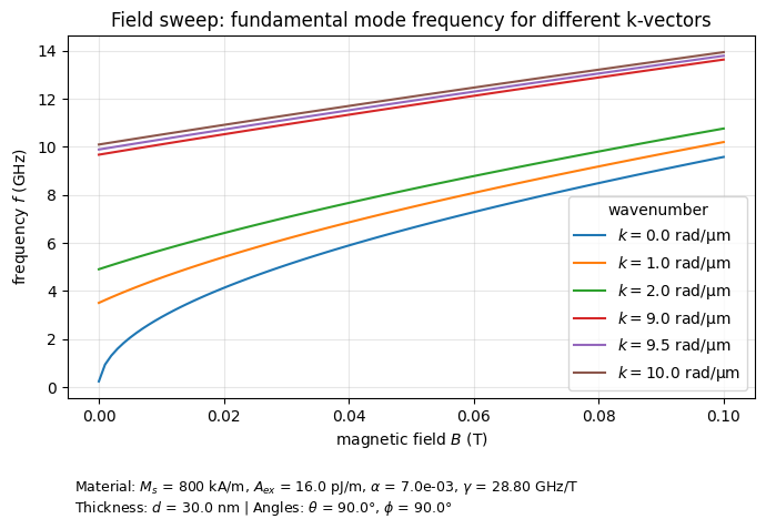
Plot the data #1

Now we can just slice our 2D arrays n0 and decay0 and plot whatever we want. Let’s start with plotting a field dependence of the fundamental mode frequency (n0 array) for different values of the k-vector.

# print what k-values we have available in k array in index:value format, separated by |
print("| ".join(f"{i}:{val/1e6:.1f}" for i, val in enumerate(k)))

0:0.0| 1:0.1| 2:0.2| 3:0.3| 4:0.4| 5:0.5| 6:0.6| 7:0.7| 8:0.8| 9:0.9| 10:1.0| 11:1.1| 12:1.2| 13:1.3| 14:1.4| 15:1.5| 16:1.6| 17:1.7| 18:1.8| 19:1.9| 20:2.0| 21:2.1| 22:2.2| 23:2.3| 24:2.4| 25:2.5| 26:2.6| 27:2.7| 28:2.8| 29:2.9| 30:3.0| 31:3.1| 32:3.2| 33:3.3| 34:3.4| 35:3.5| 36:3.6| 37:3.7| 38:3.8| 39:3.9| 40:4.0| 41:4.1| 42:4.2| 43:4.3| 44:4.4| 45:4.5| 46:4.6| 47:4.7| 48:4.8| 49:4.9| 50:5.0| 51:5.1| 52:5.2| 53:5.3| 54:5.4| 55:5.5| 56:5.6| 57:5.7| 58:5.8| 59:5.9| 60:6.0| 61:6.1| 62:6.2| 63:6.3| 64:6.4| 65:6.5| 66:6.6| 67:6.7| 68:6.8| 69:6.9| 70:7.0| 71:7.1| 72:7.2| 73:7.3| 74:7.4| 75:7.5| 76:7.6| 77:7.7| 78:7.8| 79:7.9| 80:8.0| 81:8.1| 82:8.2| 83:8.3| 84:8.4| 85:8.5| 86:8.6| 87:8.7| 88:8.8| 89:8.9| 90:9.0| 91:9.1| 92:9.2| 93:9.3| 94:9.4| 95:9.5| 96:9.6| 97:9.7| 98:9.8| 99:9.9| 100:10.0

# Choose which k-indices to plot (edit as you like, look at the k-values above)
k_indices = [0, 10, 20, 90, 95, 100]

fig, ax = plt.subplots(figsize=(7, 5))

for ki in k_indices:
    ax.plot(B, n0[:, ki], label=f"$k = ${k[ki]*1e-6:.1f} rad/μm")

ax.set_xlabel(r"magnetic field $B$ (T)")
ax.set_ylabel(r"frequency $f$ (GHz)")
ax.set_title("Field sweep: fundamental mode frequency for different k-vectors")
ax.grid(True, alpha=0.3)
ax.legend(title="wavenumber")

# --- Info box ---
info_text = (
    r"Material: $M_s$ = {:.0f} kA/m, $A_{{ex}}$ = {:.1f} pJ/m, "
    r"$\alpha$ = {:.1e}, $\gamma$ = {:.2f} GHz/T" "\n"
    r"Thickness: $d$ = {:.1f} nm | Angles: $\theta$ = {:.1f}°, $\phi$ = {:.1f}°"
).format(
    sl.Ms/1e3, sl.Aex*1e12, sl.alpha, sl.gamma/(2*np.pi*1e9),
    sl.d*1e9, np.rad2deg(sl.theta), np.rad2deg(sl.phi)
)

ax.text(
    0.01, -0.22, info_text,
    transform=ax.transAxes, ha="left", va="top", fontsize=9
)

plt.tight_layout()
plt.show()

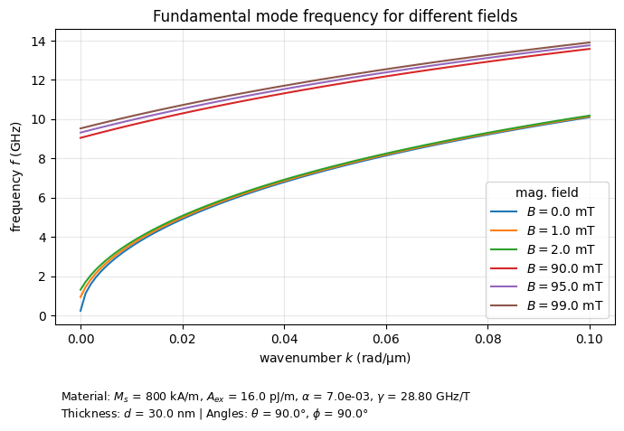
Plot the data #2

But we can also plot dispersion (frequency vs wavenumber) for different fields. Everything is already calculated in ndarray n0, we just need to plot it:

# print what B values we have available in B array in index:value format, separated by |
print("| ".join(f"{i}:{val*1e3:.1f}" for i, val in enumerate(B)))

0:0.0| 1:1.0| 2:2.0| 3:3.0| 4:4.0| 5:5.0| 6:6.0| 7:7.0| 8:8.0| 9:9.0| 10:10.0| 11:11.0| 12:12.0| 13:13.0| 14:14.0| 15:15.0| 16:16.0| 17:17.0| 18:18.0| 19:19.0| 20:20.0| 21:21.0| 22:22.0| 23:23.0| 24:24.0| 25:25.0| 26:26.0| 27:27.0| 28:28.0| 29:29.0| 30:30.0| 31:31.0| 32:32.0| 33:33.0| 34:34.0| 35:35.0| 36:36.0| 37:37.0| 38:38.0| 39:39.0| 40:40.0| 41:41.0| 42:42.0| 43:43.0| 44:44.0| 45:45.0| 46:46.0| 47:47.0| 48:48.0| 49:49.0| 50:50.0| 51:51.0| 52:52.0| 53:53.0| 54:54.0| 55:55.0| 56:56.0| 57:57.0| 58:58.0| 59:59.0| 60:60.0| 61:61.0| 62:62.0| 63:63.0| 64:64.0| 65:65.0| 66:66.0| 67:67.0| 68:68.0| 69:69.0| 70:70.0| 71:71.0| 72:72.0| 73:73.0| 74:74.0| 75:75.0| 76:76.0| 77:77.0| 78:78.0| 79:79.0| 80:80.0| 81:81.0| 82:82.0| 83:83.0| 84:84.0| 85:85.0| 86:86.0| 87:87.0| 88:88.0| 89:89.0| 90:90.0| 91:91.0| 92:92.0| 93:93.0| 94:94.0| 95:95.0| 96:96.0| 97:97.0| 98:98.0| 99:99.0| 100:100.0

# Choose which k-indices to plot (edit as you like, look at the B-values above)
B_indices = [0, 1, 2, 90, 95, 99]

fig, ax = plt.subplots(figsize=(7, 5))

for Bi in B_indices:
    ax.plot(B, n0[Bi, :], label=f"$B = ${B[Bi]*1e3:.1f} mT")

ax.set_xlabel(r"wavenumber $k$ (rad/µm)")
ax.set_ylabel(r"frequency $f$ (GHz)")
ax.set_title("Fundamental mode frequency for different fields")
ax.grid(True, alpha=0.3)
ax.legend(title="mag. field")

# --- Info box ---
info_text = (
    r"Material: $M_s$ = {:.0f} kA/m, $A_{{ex}}$ = {:.1f} pJ/m, "
    r"$\alpha$ = {:.1e}, $\gamma$ = {:.2f} GHz/T" "\n"
    r"Thickness: $d$ = {:.1f} nm | Angles: $\theta$ = {:.1f}°, $\phi$ = {:.1f}°"
).format(
    sl.Ms/1e3, sl.Aex*1e12, sl.alpha, sl.gamma/(2*np.pi*1e9),
    sl.d*1e9, np.rad2deg(sl.theta), np.rad2deg(sl.phi)
)

ax.text(
    0.01, -0.22, info_text,
    transform=ax.transAxes, ha="left", va="top", fontsize=9
)

plt.tight_layout()
plt.show()

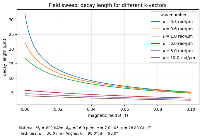
Plot the data #3

Because together with mode frequencies we’ve also calculated decay lenghts, now we can have a look at what is in decay0 ndarray.

# print what k-values we have available in k array in index:value format, separated by |
print("| ".join(f"{i}:{val/1e6:.2f}" for i, val in enumerate(k)))

0:0.00| 1:0.10| 2:0.20| 3:0.30| 4:0.40| 5:0.50| 6:0.60| 7:0.70| 8:0.80| 9:0.90| 10:1.00| 11:1.10| 12:1.20| 13:1.30| 14:1.40| 15:1.50| 16:1.60| 17:1.70| 18:1.80| 19:1.90| 20:2.00| 21:2.10| 22:2.20| 23:2.30| 24:2.40| 25:2.50| 26:2.60| 27:2.70| 28:2.80| 29:2.90| 30:3.00| 31:3.10| 32:3.20| 33:3.30| 34:3.40| 35:3.50| 36:3.60| 37:3.70| 38:3.80| 39:3.90| 40:4.00| 41:4.10| 42:4.20| 43:4.30| 44:4.40| 45:4.50| 46:4.60| 47:4.70| 48:4.80| 49:4.90| 50:5.00| 51:5.10| 52:5.20| 53:5.30| 54:5.40| 55:5.50| 56:5.60| 57:5.70| 58:5.80| 59:5.90| 60:6.00| 61:6.10| 62:6.20| 63:6.30| 64:6.40| 65:6.50| 66:6.60| 67:6.70| 68:6.80| 69:6.90| 70:7.00| 71:7.10| 72:7.20| 73:7.30| 74:7.40| 75:7.50| 76:7.60| 77:7.70| 78:7.80| 79:7.90| 80:8.00| 81:8.10| 82:8.20| 83:8.30| 84:8.40| 85:8.50| 86:8.60| 87:8.70| 88:8.80| 89:8.90| 90:9.00| 91:9.10| 92:9.20| 93:9.30| 94:9.40| 95:9.50| 96:9.60| 97:9.70| 98:9.80| 99:9.90| 100:10.00

# Choose which k-indices to plot (edit as you like, look at the k-values above)
k_indices = [3, 6, 10, 60, 80, 100]

fig, ax = plt.subplots(figsize=(7, 5))

for ki in k_indices:
    ax.plot(B, decay0[:, ki], label=f"$k = ${k[ki]*1e-6:.1f} rad/μm")

ax.set_xlabel(f"magnetic field $B$ (T)")
ax.set_ylabel("decay length (μm)")
ax.set_title("Field sweep: decay length for different k-vectors")
ax.grid(True, alpha=0.3)
ax.legend(title="wavenumber")

# --- Info box ---
info_text = (
    r"Material: $M_s$ = {:.0f} kA/m, $A_{{ex}}$ = {:.1f} pJ/m, "
    r"$\alpha$ = {:.1e}, $\gamma$ = {:.2f} GHz/T" "\n"
    r"Thickness: $d$ = {:.1f} nm | Angles: $\theta$ = {:.1f}°, $\phi$ = {:.1f}°"
).format(
    sl.Ms/1e3, sl.Aex*1e12, sl.alpha, sl.gamma/(2*np.pi*1e9),
    sl.d*1e9, np.rad2deg(sl.theta), np.rad2deg(sl.phi)
)

ax.text(
    0.01, -0.22, info_text,
    transform=ax.transAxes, ha="left", va="top", fontsize=9
)

plt.tight_layout()
plt.show()