Getting Started

Warning

Needs to be updated!

Installation

The easiest way to install SpinWaveToolkit is via pip from PyPI. To do this, open the command line and type

py -m pip install SpinWaveToolkit --user

Other installation approaches are descried in the User Guide.

Setting up the experiment

Import needed packages. For plotting, we will use matplotlib, but SpinWaveToolkit does not depend on it.

import numpy as np
import matplotlib.pyplot as plt
import SpinWaveToolkit as swt

Choose a model

First, you need to choose the appropriate model for your experiment. This depends mainly on the configuration. Currently, there are these dispersion models:

• single magnetic layer (zeroth perturbation - omits intermode coupling, mainly for thin films) - SingleLayer

• single magnetic layer with intermode coupling (useful for thicker layers) - SingleLayerNumeric

• two coupled magnetic layers (e.g. syntheric antiferromagnets) - DoubleLayerNumeric

• one magnetic layer dipolarly coupled to a superconducting layer - SingleLayerSCcoupled

• magnon-polariton in a bulk ferromagnet (very small wavevectors) - BulkPolariton

Let’s assume a single magnetic layer for the following examples. Therefore, we will use the SingleLayer class.

Define your material

To handle materials, SpinWaveToolkit uses the Material class. You can either use one of the predefined materials (see documentation of Material), or define your own by specifying its parameters

NiFe = swt.Material(Ms=800e3, Aex=16e-12, alpha=0.007, gamma=30*2e9*np.pi)

Set up geometry and conditions

Here, we will assume a 30 nm thick film in an in-plane external field of 10 mT. We will calculate the dispersion for wavevectors up to 30 rad/µm in the direction perpendicular to the magnetization (i.e. Damon-Eshbach geometry). For simplicity, totally unpinned spins at the boundaries are assumed.

Bext = 10e-3  # (T) magnetic field
d = 30e-9  # (m) thickness of the layer
k = np.linspace(0, 30e6, 200)+1  # (rad/m) wavevector range (+1 to avoid NaN at k=0)
theta = np.pi/2  # (rad) angle of magnetization from thin film normal
phi = np.pi/2  # (rad) angle of wavevector from in-plane magnetization
bc = 1  # boundary condition (1 for totally unpinned)

# initialize the model
sl = swt.SingleLayer(Bext, NiFe, d, k, theta, phi, boundary_cond=bc)

Retrieve dispersion relation

To calculate the dispersion relation, simply call the SingleLayer.GetDispersion() method of the model instance. This will return the frequencies of the spin wave modes in rad/s (angular frequency), but spin waves are usually studied in the GHz frequencies.

f = sl.GetDispersion() / (2e9 * np.pi)  # rad/s to GHz

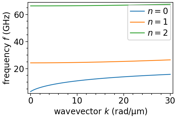
In this model, we can also simply calculate higher-order perpendicular standing spin wave (PSSW) modes by specifying the mode number as an argument to SingleLayer.GetDispersion(). For example, to get the first three modes

f0 = sl.GetDispersion(n=0) / (2e9 * np.pi)  # fundamental mode (same as `f` above)
f1 = sl.GetDispersion(n=1) / (2e9 * np.pi)  # first PSSW mode
f2 = sl.GetDispersion(n=2) / (2e9 * np.pi)  # second PSSW mode

or more concisely

modes = np.array([sl.GetDispersion(n=i) / (2e9 * np.pi) for i in range(3)])

which can be then easily plotted e.g. as

for i in range(3):
    plt.plot(k*1e-6, modes[i], label=f"$n={i}$")
plt.xlabel(r"wavevector $k$ (rad/µm)")
plt.ylabel(r"frequency $f$ (GHz)")
plt.legend(loc="lower right")

Calculate other quantities

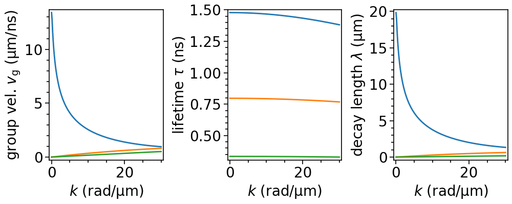
Similarly to the dispersion relation, other quantities can be calculated. For example, the group velocity can be obtained by calling SingleLayer.GetGroupVelocity(). Analogically, the lifetime and decay length are retrieved. Those are numerically calculated based on the dispersion relation for the given PSSW mode.

...
vg = sl.GetGroupVelocity(n=0)*1e-3  # m/s to um/ns
tau = sl.GetLifetime(n=0)*1e9  # s to ns
lam = sl.GetDecLen(n=0)*1e6  # m to um
...

Note

The methods for dispersion relation, group velocity, lifetime, and decay length are usually implemented in all dispersion models with a similar syntax. For exact syntax and full list of the supported methods, refer to the appropriate class documentation.

Change parameters

With the instance of the respective model, it is simple to change individual parameters, as most of them are also accessible at attributes of the same name as the input parameters. For example to change now to backward volume spin waves, just change the in-plane angle phi of our SingleLayer instance.

sl.phi = 0  # change to 0 rad
f_bv = sl.GetDispersion()/2e9/np.pi

Sweeps

This can be further used to make sweeps of certain parameters. Here we show a field sweep of the dispersion relation in the sample defined above.

nfields = 100
fields = np.linspace(0, 100e-3, nfields)  # (T) field vector
f_sweep = np.empty((nfields, k.shape[0]))  # preallocated array for dispersion
for i in range(nfields):
    sl.Bext = fields[i]
    f_sweep[i] = sl.GetDispersion()/2e9/np.pi

---

That’s it! You have learned the basic usage of the SpinWaveToolkit! Now you can head over to the User Guide and Examples for more tutorials. If you encounter any problems, see the appropriate topic in the API reference or let us know in the Discussions on GitHub.